MPI Fortran 90 programs on Dense Matrix Computations ( Vector - Vector, Matrix -Vector, Matrix-Matrix Multiplication) are considered for execution on Message Passing Cluster or Multi Core Systems that support MPI library.

Fortran 90 program to print Hello World program.

Fortran 90 program to print Welcome Message .

Fortran 90 program to find equation of line joining two distinct points .

Fortran 90 program to compute Matrix-Vector multiplication using intrinsic function MATMUL ( Use Math Library function)

Fortran 90 program to find root of a quadratic equation.

Fortran 90 program for Least Square Approximation method.

Fortran 90 program to find the roots of equation f(x) = 0 using Newton Raphson method.

Fortran 90 program to solve a system of linear equations Ax = b using Gaussian Elimination method.

Fortran 90 program to compute Matrix and Matrix Multiplication using block checkerboard partitioning and Cannon Algorithm. (Assignment)

Write an MPI fortran90 program performing MPI I/O to single file (Using MPI 2.0).

Example 1 : Description of Implementation of Fortran 90 Program to print Hello World!

• Objective

Write a simple Fortran 90 program to print "Hello World!".

• Description

This program prints the message  "Hello World!" on screen when it executes.

• Input

None

• Output 

Message "Hello World!".

Example 2 : Description for implementation of Fortran 90 program to print Welcome Message

• Objective

  Write a simple Fortran 90 program to print which asks user his/her title, first name and last name, and prints a welcome message using both full name and first name.

• Description

This program performs simple character manipulation. However, there are some slight difficulties in combining the title, first and last names in a form which will avoid multiple spaces within the composite name. The most useful intrinsic procedure TRIM is used. TRIM removes any trailing blanks from the character string provided as its argument. Notice that TRIM has been used in the second PRINT statement to ensure that the question mark at the end of the question comes immediately after the name, and not separated from it by several spaces.

• Input

  Title, first name and last name of an user.

• Output 

Welcome message using both full name and first name.

Example 3 : Description for implementation of Fortran 90 program to find equation of line joining two distinct points.

• Objective

Write Fortran 90 program to calculate equation of line from given two distinct points.

• Description :

Each process reads respective input array of different size n/p from the given input file. The process wit rank 0 accumalates the total number of integers to be recevied from the each process and allocates memory for the output integer array and performs MPI_gatherv operation.

A straight line is defined by an equation of the form ax + by + c = 0 and at first sight we could simply use the three coefficients of this equation as the representation of a line. However these three coefficients are not unique.



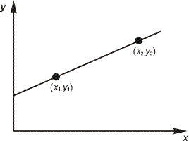
 Figure 1 : Line joining two distinct points




The slope of the line is (y₂ - y₁)/(x₂ -x₁) if x₁ is not equal to x₂.

"At any point (x, y) other than (x₁, y₁), the slope is (y - y₁) / (x - x₁).

Therefore equation of line becomes

(x₂ - x₁)(y - y₁) = (y₂ - y₁)(x - x₁)                                         (1)

Rearranging equation (1) we have

 (y₂ -  y₁)x + (x₁- x₂)y - y₂x₁ + y₁x₁ + y₁x₂ - y₁x₁ = 0

Therefore

a =   y₂ - y₁         b =   x₁ - x₂         c =   y₁x₂ - y₂x₁

In this example we have defines two data types, one to represent a point by means of its coordinates in two dimensional space only and the other to represent a line which is also in two dimensional space by the coefficients of its defining equation. We have assumed that the user does not supply two identical points.

• Input

Coordinates of two distinct points.

• Output 

Equation of line joining two distinct points.

Example 4 : Description for implementation of Fortran 90 program to compute Matrix-Vector multiplication using intrinsic function MATMUL

• Objective

Write a Fortran 90 program for matrix-vector multiplication using intrinsic function MATMUL

• Description

Fortran 90 provides some intrinsic functions specifically designed for vector and matrix operations, where it is assumed that matrices are stored in two dimensional arrays and vectors are stored in one dimensional arrays.. Fortran 90 contains a large number of other intrinsic functions which operate on arrays of any dimension. In this example Matrix_A and Vector are allocated using ALLOCATE statement. ALLOCATE statement dynamically allocates space for an allocatable array. Intrinsic function MATMUL is used to perform matrix and vector multiplication and the resultant vector is stored in C. Currently allocated arrays are deallocated by the related DEALLOCATE statement. The DEALLOCATE statement has the effect of changing its atatus to not currently allocated and making the memory space that it was using available for other purpose.

• Input

Size of the matrix and Vector

• Output 

Output Vector

Example 5 : Write f90 Program to find roots of a quadratic equation

• Objective

Write a MPI program to gather values from each process and store the output values in the global integer array A of dimension n on p process of cluster. Use MPI_AllgatherCommunication library call in the program.

• Description
On the surface, finding root of a quadratic equation, appears to be a simple problem. However, even such a simple problem involves subtle numerical issues if we are trying to produce a robust software. Consider simple quadratic equation

ax² + bx + c = 0 

where a is not equal to zero, has two roots, given by the formula



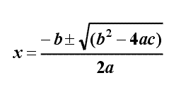
It is immediately apparent that there are three possible cases:

(1) b² > 4ac in which case the equation will have two real roots.

(2) b²  = 4ac in which case the equation will have one root (or two coincident roots)

(3) b² < 4ac in which case the equation will have no roots (or at least no real roots, and we are not concerned with imaginary roots in this program.

In this example we have demonstrated the use of CASE statement. However there are two major difficulties. The first of these is that the values of the coefficients in this sort of problem will normally be real, and therefore the expression b² < 4ac is also real. But the case_expression in a CASE statement must be integer, character or logical. 

The other problem concerns with case 2, where the value of the expression is 0. In particular we should never compare two real numbers for equality, as two numbers which are mathematically equal will often differ very slightly if they have been calculated in a different way. This difficulty is avoided by comparing the difference between two real numbers with a very small number. Thus the second case can be rewritten as

|b² - 4ac| < epsilon

In this program we have dealt with both these problems at the same time by dividing the value of b² - 4ac by epsilon and then assigning the result to an integer for use in CASE statement. This means that if |b² - 4ac| < epsilon the result off the division is between -1 and +1, and the integer stored, as a result of truncation is 0. If b2 - 4ac > epsilon then the result stored is positive integer, while b² - 4ac < epsilon the result stored is negative integer. We have assumed that a is a non-zero value.

• Input

Coefficients of a quadratic equation where a is non-zero value.

• Output 

Roots of a quadratic equation.

Example 6 : Description for implementation of Fortran 90 program for Least Square Approximation method.

• Objective

Write Fortran 90 program for Least Square Approximation method. Write a Fortran 90 program to calculate the value of Young's modulus of given material and the natural length of the wire using Least Square Approximation method

• BackGround & Description

Data fitting by least square Method
A frequent situation in experimental sciences is that data has been collected which it is believed, will satisfy a linear relationship of the form

y   =  ax + b

However, due to experimental error, the relationship between the data collected at different times will rarely be identical, and can typically be represented graphically as shown in Figure 2. Fitting a straight line through the data in such a way as to obtain the fit which most closely reflects the true relationship is therefore, a widespread need. One well-established method is known as the method of least squares.



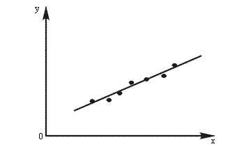
Figure 2 : Experimental data which exhibits a linear relationship.



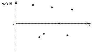
Figure 3 : Residuals for the data from Figure 2



This method can be applied to any polynomial, or even to more general functions, but for the present we shall only consider the linear case. If we assume that the equation

y = ax + b

is a possible best fit then we can test its accuracy by calculating the predicted values of y for the actual data values of x and comparing them with the corresponding data values. The difference between a calculated value y' and and experimental value y is called the residual, and the method of least squares attempts to minimize the sum of the squares of the residuals for all the data points. Figure 3 shows the residuals for the data in Figure 2 in graphical form, and it can easily be seen that using the square of the residuals eliminates the problem caused by some predicted values being too large and others being too small.


• Description

In this example the extensions produced in the wire by suspending various weights from it were measured very accurately. Young's modulus is defined by the equation

      E = stress / strain

which can be expressed as 

     E=(f /A) / (e / L)    or    E = (fL) / Ae

where f is the applied force (the weight), A is the cross-sectional area of the wire (measured at several points and averaged), e is the extension, and L is the unstressed length of the wire.

In this case, in order to eliminate the effect of any curl or kinking in the wire no measurements were taken in a completely unstressed condition, but the length of the wire was measured instead under an initial load and then under various heavier loads.

From the above definition of Young's modulus we can derive the equation

    e = kf       where      k = L / AE

However, we do not have the value of e, but rather the value of  l, where

e = l - L

We therefore need to fit the equation

l = kf + L

to the experimental data. We shall then be able to calculate the value of E.

In accordance with good practice all the constants required for problem are placed in a module so that they can be easily accessed from any procedure in the program. 

In this example we have used SUM and DOT_PRODUCT  intrinsic functions.

• Input

Read length of a wire under various load from a file least_sq.inp which is as follows.
9
10 39.967
12 39.971
15 39.979
17 39.986
20 39.993
22 40.000
25 40.007
28 40.016
30 40.022
0.025


• Output

Value of Young's modulus and natural length of wire.

Example 7 : Description for implementation of Fortran 90 program to find the roots of equation f(x) = 0 using Newton Raphson method.

• Objective

Write a fortran 90 program to find root of equation f(x) = 0 using Newton Raphson method.

• BackGround & Description

f(x) at the end points of the interval, but not the value of f(x) at those points. Another weakness is that, for the method to work at all, the initial two points must be bracket a root. 

It is possible to combine interval-bisection with such faster methods and retain much of the best of both worlds, namely fast convergence and guaranteed convergence.

• Description 

Newton's method, sometimes known as the Newton-Raphoson method. This method uses not only function values but also approximation. Figure 4 shows how, given the gradient at a point x_i, it is easy to obtain a new estimate for the root. In this method, we do not bracket a root by an interval but, instead, generate a sequence of approximation that if successful tend to the root.



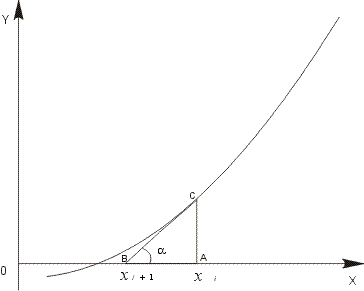
Figure 4 : Newton Raphson Approximation
From Figure 4 we can readily see that

x_i+1     =   OB       = OA-AB       = x_i - AB       = x_i - (AC / tan a )
          =   x_i - (f(x_i) / f '(x_i))


where f ^'(x_i) is the gradient of the curve at the point C, ((x_i, f '(x_i)), which is equal to tan a.

This formula

x_i+1 = x_i - (f(x_i) / f '(x_i)

is known as Newton's iteration, and is the basis for Newton' method of approximation to a root.
An external function is used to define the equation and its first derivative

• Input
X-coordinate of the point which can be used as the starting point for the interpolation and number of iterations.
• Output

Estimated value of root and its first derivative.

Example 8 : Description for implementation of Fortran 90 program to solve a system of linear equations Ax = b using Gaussian Elimination method.

• Objective

Write a fortran 90 program to solve a system of linear equations Ax = b using Gaussian elimination method.

• BackGround & Description

  The system of linear equations [A]{x} = {b} is given by 

  a_0,0 x₀ + a_0,1 x₁ + ...+ a_{0, n-1} x_n-1 = b₀ , 
  a_1,0 x₀ + a_1,1 x₁ + ...+ a_{1, n-1} x _n-1 = b₁ ,  
  ...........................................................................  
  ........................................................................... 
   ...........................................................................  
  a_n-1,0 x₀ + a_n-1,1 x₁ + ...+ a_{n-1, n-1} x _n-1 = b_n-1 . 

  In matrix notation, this system of linear equation is written as [A]{x}={b} where A[i, j] = a_{i, j} , b is an n x 1 vector [b_o,b₁,...,b_n-1]^T, and is the desired solution vector [x_o,x₁,...,x_n-1]^T. We will make all subsequent references to a_{i, j} by A[i, j] and x_i by x[i ].  

  Iterative methods are techniques to solve systems of equations of the form [A]{x}={b} that generate a sequence of approximations to the solution vector x. In each iteration, the coefficient matrix A is used to perform a matrix-vector multiplication. The number of iterations required to solve a system of equations with a desired precision is usually data dependent; hence, the number of iterations is not known prior to executing the algorithm. Therefore, we can analyze the performance and scalability of a single iteration of an iterative method. Iterative methods do not guarantee a solution for all systems of equations. However, when they do yield a solution, they are usually less expensive than direct methods  for matrix factorization for large size of matrices.

• Description 

Suppose we have a system of n linear equations in n unknowns:

a_1,1x₁ + a_1,2 x₂ +...... + a₁,_nx _n = b₁

a_2,1x₁ + a_2,2x₂ + ...... + a₂,_nx _n = b₂

..........................................................  
................................................................  

a_n,1x₁ + a _n,2x₂ + ...... + a_n , _nx_n = b_n

Gaussian elimination will turn this system of equations into an equivalent system of equations of the form

c _1,1x ₁ + c _1,2 x ₂ + ...... + c _1,nx_n = d


c _2,2 x₂ + ...... + c_2,nx_n = d_2
.
.
.
c_{n, n}x_n = d _n

In this form, all the coefficients below the diagonal are zero, and the matrix of coefficients, for obvious reasons, is said to be upper triangular. As we shall see, in this form, the system of equations can be solved with no further manipulation. Gaussian elimination works by subtracting multiples of the first equations from all the other equations below it in such a way that the resulting equations each have a coefficient of 0 for x₁. Thus, the initial system of equations becomes

a_{1, 1}x₁ + a_{1, 2}x₂ + ...... + a_{1, n}x_n = b₁
a⁽¹⁾_{2, 2}x₂ + ...... + a⁽¹⁾_{2, n}x_n = b^{( 1 )}₂
a⁽²⁾_{2, 2}x₂ +...... + a⁽²⁾_{2, n}x_n = b^{( 2 )}  ₂
.
.
.
a⁽²⁾_{n, 2}x₂ + ...... + a⁽¹⁾_{n, n}x_n = b^{( 2 )}  _n

Specifically, for  j greater or equal to 2, the j^th the equation is obtained by subtracting the first equation, multiplied by from the original equation. The superscripts on the coefficients are used to denote that this is step I of the process. The solution of the second set of equations is the same as that of the original system of equations.

We now repeat the process again on the (n - 1) * (n - 1) system of equations consisting of the second to the n^th equations. Subtracting appropriate multiples of the second equation from the equations below it, we obtain a system of equations in which all the equations after the second have zero for the coefficient of x₂.

Proceeding iteratively, after n-1 steps, we obtain a system of equations of the form

a_1,1x₁ + a_1,2x₂ + a_1,3x₃ + a_1,4x₄ +  ......+ a_1,n-1x_n-1 + a_1,nx_n = b₁
a⁽¹⁾_2,2x₂ + a⁽¹⁾_2,3x₃ + a⁽¹⁾_2,4x₄ + ...... + a⁽¹⁾_2,n-1x_n-1 + a⁽¹⁾_2,nx_n = b^{(  1 )} ₂
a⁽²⁾_3,3x₃ + a⁽²⁾_3,4x₄ +  ...... + a⁽²⁾_3,n-1x_n-1 + a⁽²⁾_3,nx_n  = b^{(  2  )}₃
a⁽³⁾_4,4x₄ + .+ a⁽³⁾_4,n-1x_n-1+ a⁽³⁾_4,nx_n= b^{(  2  )}_4
.
.
.
a^{(n - 2)}_n-1,n-1x_n-1 + ...... + a^{(n - 2)}_n-1,nx_n= b^{(n - 2)}_n-1
a^{(n - 1)}_n,nx_n= b^{(n - 1)}_n

This process is called Gaussian elimination, and the a_i,i ^(i-1)(the element along the diagonal) are called pivots.

Now the n^th equation is solved for x_n by dividing by a_n,n^(n-1). This value is then substituted into the (n - 1)^th equation, which can then be solved for (x_{n -1}). The values for x_n and x_n-1 are substituted in the (n-2)^th equation. which is then solved for x_n-2. We proceed backwards through the set of equations in this way until we finally put the values determined for x_n, x_n-1, ...x₃,x₂ into the first equation and solve it for x₁. This processed, for obvious reasons, is called back substitution. 

We can see that the Gaussian elimination process will fail if, at the i^th step, the coefficient a_i,i^(i-1) is 0. We would in this case be unable to make all the coefficients of x_i in the equations below it 0, since subtracting any multiple of 0 leaves a number unchanged. If this situation occurs, however, we could interchange the i^th equation with one below it that does not have a 0 for the coefficient of xi, and then proceed. If there is no such equation, then it can be proved that the original system either has no solution or an infinite set of solutions. Observe that changing the order of occurrence of the equations does not change their solution.

In fact, we can go somewhat beyond this interchange procedure. If a pivot element is small, then large multiples of the equation containing it must be used during the elimination process. This will multiply any errors (due to round-off effects) in the other coefficients of this equation. Intuitively, we can see that this is undesirable. So, for reasons of numerical stability, at the beginning of the i^th step, we will reorder the equations from the i^th one down, so that one that has the largest absolute value for the coefficient of x_j becomes the i^th equation. 

In this program two subroutines 'gaussian_elemination' and 'back_substitution' are called by another subroutine 'gaussian_solve'. We do not want a user to be able to call 'gaussian_elimination' or 'back_substitution' directly. As well as the subroutine 'gaussian_solve' will use assumed-shape dummy arguments, it must have an explicit interface in the main program. To accomplish both of these aims, all three subroutines are put in a module called 'Linear_Equations' being public

• Input

Read Matrix and vector from file gauss.inp which is as below.

4
8 3 1 1
1 4 2 1
1 6 2 2
3 1 3 8
5
1
5
4


• Output

Solution x of matrix system Ax = b.

Example 9 : Description for implementation of MPI program to compute Matrix Matrix Multiplication using block checkerboard partitioning and Cannon Algorithm. (Assignment)

• Objective

Write a fortran 90 program to compute Matrix Matrix Multiplication using block checkerboard partitioning and Cannon Algorithm

• Objective 

  Write a f90 program, for computing the matrix-matrix multiplication on p on Single core or SMP System. Use block checkerboard partitioning of the matrices and Cannon's Algorithm. 

  Assume that size of the square matrices i.e.   p= q² and the size of square matrices A and B is evenly divisible by q.  It is assumed that the number of blocks are equal to the number of processors as explained in Cannoon's Algorithm

• Description 
  

  Cannon's algorithm is based on cartesian virtual topology. Assume that A and B are square matrices of size n and C be the output  matrix. These matrices are dived into blocks or submatrices to perform matrix-matrix operations in parallel .For example, an n x n matrix A can be regarded as q x q array of blocks A_{i, j} (0<=i <q, 0<= j < q) such that each block is an (n/q) x (n/q) submatrix. We use p processors to implement the block version of matrix multiplication in parallel by choosing q as a square root of  p  and compute a distinct block C_{i, j} on each processor. Block  and cyclic checkerboard partitioning of a 8 x 8 matrix on a square grid (4  x 4) of processors is shown in the Figure 5 
  

  

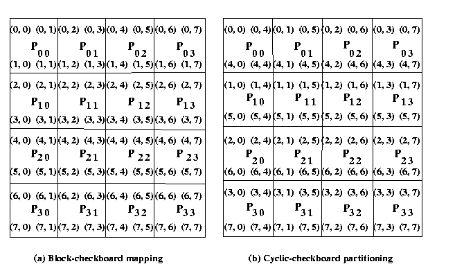
                            Figure 5 : Checkerboard partitioning of 8 x 8 matrices on 16 processors. 

  The matrices A and B are partitioned into p  blocks, A _{i, j} and B _{i, j} (0<=i < q, 0<= j < q) of size  (n/q x n/q)   on each process. These blocks are mapped onto a q x q  logical mesh of processes. The processes are labeled from P_0,0 to P_q-1,q-1. An example of of this situation is shown in Figure 14  Process P_{i, j} initially store block matrices A_{i, j} and B_{i, j} and computes block C_{i, j} of result matrix. To compute submatrix C_{i, j} , we need all submatrices , A_{i, k} and  B_{k, j} ( 0 <= k < q ) . To acquire all the required blocks, an all-to-all broadcast of matrix A_{i, j} 's  is performed in each row and similarly in each column of matrix B_{i, j}'s. MPI collective communication is used to perform this operations.

  After P_{i, j} acquires, A _i,0 , A _i,1 , A _i,2 , A _{i, q-1} and B_{0, j} , B_{1, j} , B_{2, j} , B_{q-1, j} , it performs the serial block matrix to matrix multiplication and accumulates the partial block  matrix C_{i, j} of matrix C . To obtain the resultant product matrix C, processes with rank 0 gathers all the block matrices by using MPI_Gather collective communication operation.

   MPI provides a set of special routines to virtual  topologies. An important virtual  topology is the Cartesian topology . This is simply a decomposition in the natural co-ordinate ( e.g., x,y,z) directions.

  As discussed above, there are p processors arranged in q x q square grid of processors and the input matrices, A and B are distributed among the processes in checkerboard fashion. It results in constructing p block matrices of A and B. It uses only point-to-point communication for circularly shifting blocks of matrix A and matrix B among p processes. 

  The algorithm proceeds in q stages. The first step in this algorithm is to perform initial alignment of the block matrix A and block matrix B. The blocks of matrix A are circularly shifted to the i positions to left in the row of the square grid of processes, where i  is the row number of the process in the mesh. Similarly, blocks of matrix B are circularly shifted j positions upwards, where j is the column number of the process in the processes mesh.  This operation is performed by using MPI_Sendrecv_replace .  MPI_Send and MPI_Recv is not used for point-to-point communication, because if all the processes call MPI_Send or MPI_Recv in different order the deadlocked situation may arise . 

  The algorithm performs the following steps in each stage : 

  1. Multiply the block of matrix A and matrix B and add the resultant matrix to get the block matrix C, 
      which is initially set to zero. 
  2. Circularly shift the blocks of matrix A to left in the rows of the processes and the blocks of 
       matrix B upwards in the columns of the square grid of processes in a wrap around manner. 

  The communication steps for 4 x 4 square grid of processors mesh are explained in the Figure 6. 
  

         

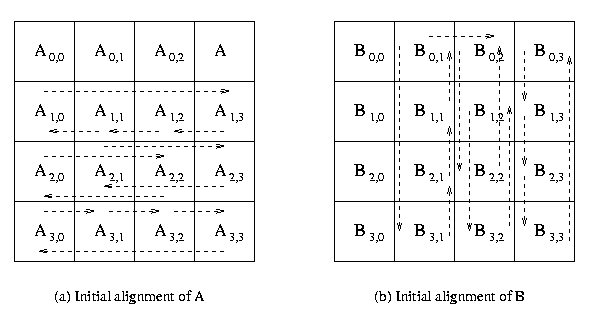
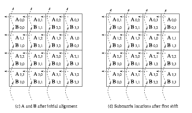
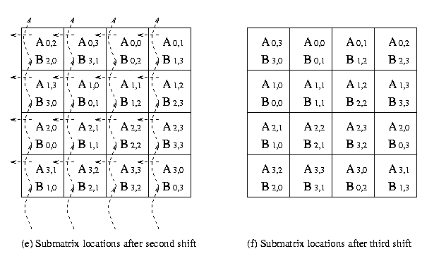
  Figure 6 :  The communication steps in Cannon's Algorithm on 16 processors. 

• Input

Assume A and B are real square matrices of size n . The input matrices are A and B. Format for the input file is given below.

The input file for the matrices A and B should strictly adhere to the following format.
#Line 1 : Number of Rows (n);   Number of columns(n). 
#Line 2 : (data) (in row-major order. This means that the data of second row follows that of the first and so on.)

• Input file &

Input file 1
A sample input file for the matrix A (8 x 8) is given below 

8    8  
1.0    2.0    3.0     4.0     2.0     3.0     2.0     1.0 
2.0    3.0    4.0     2.0     3.0     2.0     1.0     1.0 
3.0    4.0    2.0     3.0     2.0     1.0     1.0     1.0 
4.0    2.0    3.0     2.0     1.0     1.0     4.0     2.0 
2.0    3.0    2.0     1.0     2.0     3.0     2.0     2.0 
3.0    2.0    1.0     1.0     2.0     1.0     1.0     1.0 
2.0    1.0    4.0     3.0     2.0     1.0     3.0     3.0 
4.0    1.0    2.0     1.0     2.0     3.0     4.0     3.0 

Input file 2


A sample input file for the matrix B (8 x 8) is given below 

8   8  
1.0    2.0    3.0     4.0     2.0     1.0     2.0     1.0 
1.0    2.0    3.0     4.0     2.0     1.0     2.0     1.0 
1.0    2.0    3.0     4.0     2.0     1.0     2.0     1.0 
1.0    2.0    3.0     4.0     2.0     1.0     2.0     1.0 
1.0    2.0    3.0     4.0     2.0     1.0     2.0     1.0 
1.0    2.0    3.0     4.0     2.0     1.0     2.0     1.0 
1.0    2.0    3.0     4.0     2.0     1.0     2.0     1.0 
1.0    2.0    3.0     4.0     2.0     1.0     2.0     1.0 


• Output 

Prints final matrix-matrix product matrix C. The output of the matrix - matrix multiplication is given below :

18.0   36.0   54.0   72.0   36.0   18.0    36.0   18.0 
18.0   36.0   54.0   72.0   36.0   18.0    36.0   18.0 
17.0   34.0   51.0   68.0   34.0   17.0    34.0   17.0 
19.0   38.0   57.0   76.0   38.0   19.0    38.0   19.0 
17.0   34.0   51.0   68.0   34.0   17.0    34.0   17.0 
12.0   24.0   36.0   48.0   24.0   12.0    24.0   12.0 
19.0   38.0   57.0   76.0   38.0   19.0    38.0   19.0 
20.0   40.0   60.0   80.0   40.0   20.0    40.0   20.0 

Example 10 : Write an MPI fortran90 program performing MPI I/O to single file (Using MPI 2.0)

• Objective

Write an MPI program performing MPI I/O (Writing) to single file (Using MPI 2.0).

• Description

MPI process share a single file instead of the writing to seperate files, thus avoiding the having multiple files. This shows performance advantages of parallelism adopted using MPI. The new library calls of MPI are used to sharing a a file among processes. Here, MPI_COMM_WORLD libray call is used instead of MPI_COMM_SELF libray call. This indicates that all the processes are opening a single file together and it is a collective operations on the communicator, on all pariticpating process.

• Input

The input file holding the square matrix (Number of Rows, Columns of the matrix)

• Output

Single Output file