hyPACK-2013 Mode-2 : GPU Comp. CUDA enabled NVIDIA GPU Prog.

NVIDIA\92s Compute Unified Device Architecture (CUDA) is a soft- ware platform for massively parallel high-performance computing on the company's powerful GPUs. NVIDIA\92s software CUDA programming model effectively use GPUs which could be harnessed for tasks other than graphics, achieving teraflops of computing power. CUDA Programming model automatically manages the threads and it is significantly differs from single threaded CPU code and to some extent even the parallel code. Efficient CUDA programs exploit both thread parallelism within a thread block and coarser block parallelism across thread blocks. Because only threads within the same block can cooperate via shared memory and thread synchronization, programmers must partition computation into multiple blocks.

• Objective

  Write a CUBLAS CUDA program to solve the Poisson equation with Dirichlet boundary conditions in two space dimensions by finite difference method on structured rectangular type of grid. Use Jacobi iteration method to solve the discretized equations.
  

• Description

In the Poisson problem, the FD method is imposed a regular grid on the physical domain. The resuting disretized equations are solved using Jacobi Itertaive method. The description of the problem is discussed in Example 5.2

• Objective

  Write a CUBLAS CUDA program to solve the Poisson equation with Dirichlet boundary conditions in two space dimensions by finite difference method on structured rectangular type of grid. Use Jacobi iteration method to solve the discretized equations.
  

• Description

In the Poisson problem, the FD method is imposed a regular grid on the physical domain. It then approximate the derivative of unknown quantity u at a grid point by the ratio of the difference in u at two adjacent grid points to the distance between the grid point. In a simple situation, consider a square domain discretized by n x n grid points, as shown in the Figure 1(a). Assume that the grid points are numbered in a row-major order fashion from left to right and from top to bottom, as shown in the Figure 1(b). This ordering is called natural ordering . Given a total of n² points in the domain n x n grid, this numbering scheme labels the immediate neighbors of point i on the top, left, right, and bottom point as i - n, i -1, i +1 and i+n , respectively. Figure 1(b) represents partitioning of mesh using one dimensional partitioning



  Figure 1(a). Finite difference grid: Five point stencil approximation 

  Figure 1(b). One dimensional decomposition for 2-D problem, with n=7


• Formulation of Poisson Problem 

The Poisson problem is expressed by the equations

      Lu  =  f(x, y)  in the interior of domain [0,1] x [0,1]

Where L is Laplacian operator in two space dimensions.

      u(x,y)  =  g(x,y) on the boundary of the domain [0,1] x [0,1] 

We define a square mesh (also called a grid) consisting of the points (x_i , y_i), given by 

           x_i = i / n+1, i=0, ..., n+1, 

           y_j = j / n+1, j=0, ...,n+1, 

where there are n+2 points along each edge of the mesh. We will find an approximation to u(x , y) only at the points (x_i, y_j). Let u_{i, j} be the approximate solution to u at (x_i, y_j). and let h = 1/(n+1). Now, we can approximate at each of these points with the formula 

   (u_{i-1, j} +u_{i, j+1}+u_{i, j-1}+u_{i+1, j}-4u_{i, j} )/ h² = f_{i, j} . 



Rewriting the above equation as 
   u_{i, j} = 1/4(u_{i-1, j}+u_{i, j+1}+u_{i, j-1}+u_{i+1, j}-h²f_{i, j}), 

Jacobi iteration method is employed to obtain final solution starting with initial guess solution u_i,j^k for k=0 for all mesh points u _i,j  and solve the following equation iteratively until the solution is converged. 

   u_{i, j}^k+1 = 1/4(u_{i-1, j}^k+u_{i, j+1}^k+u_{i, j-1}^k+u_{i+1, j}^k-h²f_{i, j}). 

The resultant discretized banded matrix is shown in the Figure 2.




• Implementation:

  Two implementations have been done, one using kernels written in CUDA and the other using CUBLAS library. The steps in both implementations are the same, only the API may differ.
  
  Step1: Four arrays are required for computation, one for the storing old values of U i.e Uold, one for the storing new values of U i.e Unew and one each for the storing difference between these two and storing the index values of the interior points. Memory for these are allocated on the Host and they are initialized.
  
  Step2:Four more similar arrays are allocated on the GPU (device). The values of the arrays in the host machine are copied on to the arrays allocated on the device.
  
  Step3: We begin the computation with an initial solution of all zero's for the Uold vector in the first iteration and then apply boundary conditions on both Uold and Unew by setting the boundary values at corresponding positions.
  
  Step4: We compute the Unew values by ui, j = 1/4(ui-1, j+ui, j+1+ui, j-1+ui+1, j).
  
  Step5: Next we compute the difference between Unew and Uold.
  
  Step6: We assign Unew to Uold.
  
  Step7: The values thus obtained (Uold) is used in the next iteration and steps 4,5,6 are repeated until Maximum difference value < TOLERANCE or present iteration equals Maximum iterations. All computations are done on GPU(device).
  

• CUDA API used:

  Allocates memory on device :
  
  cudaMalloc(void** array, int size)
  
  Frees memory allocated on device
  cudaFree(void* array)
  
  Copies from host to device
  
  cudaMemcpy((void*)device_array, (void*)host_array, size , cudaMemcpyHostToDevice)
  
  Copies from device to host
  
  cudaMemcpy((void*)host_array, (void*)device_array, size , cudaMemcpyDeviceToHost)
  
  Multiplies vector X by scalar alpha and adds results to vector Y and it stores result to vector Y
  
  void cublasSaxpy (int n, float alpha, const float *x, int incx, float *y, int incy)
  
  Finds the smallest index of the maximum magnitude element of vector x
  
  int cublasIsamax (int n, const float *x, int incx)
  
  Copies the vector x to the vector
  
  void cublasScopy (int n, const float *x, int incx, float *y, int incy)
  
  

• Performance:

  The gettimeofday() function which is part of sys/time.h is used to measure the time taken for computation. It is computed at the beginning of the computation and also at the end of the computation. The actual time is difference of both.
  
  

• Input

The input to the problem is given as arguments in the command line. It should be given in the following format ; Suppose that the number of points in the X direction is m, the number of points in the Y direction is n and the maximum number of iterations the program can is run is p, then the program must be run as,

       ./program_name m n p

CPU assigns the boundary values for the Uold and Unew vectors.

• Output

CPU prints the final Unew vector which is the solution to the Poisson equation with the above stated boundary values

• Objective

  Write a CUBLAS CUDA program to implement Laplace Edge Detection algorithm on CUDA enabled NVIDIA GPU with MPI as host-CPU Programming. Assignment
  

• Description

The Laplacian image kernel is a 3 x3 two-dimensional array and this kernel is applied to each pixel in the image and takes into account the pixel\92s neighbors in a 3 x 3 area around it. The organization of multidimensional thread blocks of images into multidimensional grids are required for CUDA development to process the of arrays of data in typical edge detection algorithm. This representation of data in these forms are usually best suited for migration to CUDA for processing. Such data types include images that can be represented as a two-dimensional matrix where each entry corresponds to a single pixel in the image. An image pixel consists of a discrete red, green, and blue component in the range [0 . . . 255].

We create a two-dimensional grid that is overlaid on the image, segmenting it into several rectangular sections, as illustrated in Figure 1. For simplicity, we assume the image can be evenly divided into full sized segments. In other words, the image is divided into thread blocks of 8 x 8 and 16 x 16 sizes. Each thread within the thread block corresponds to a single pixel within the image. In implementation, each thread is responsible for loading one pixel or the block of 3 x 3 pixel area into shared memory





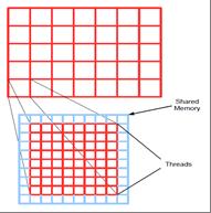
  Figure 1(a). Thread blocks for single pixel per thread method  

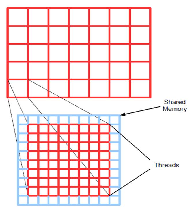
  Figure 1(b). Thread blocks for multiple pixels

For edge detection, the each target pixel requires that a 3x3 area surrounding pixels and these are analyzed to calculate the output. Therefore, threads on the edge of a thread block must examine pixels that are outside the dimensions of the thread block. In order to ensure accuracy of the output image, these threads are responsible for loading the pixels they are adjacent to that do not have a mapping in the thread block into shared memory.

That is, the threads on the edge of the block load the boundary pixels into shared memory. This extra step is performed after the initial shared memory load that all threads perform. To compensate for the required extra space, the two-dimensional shared memory array is allocated to have dimensions of (blockDim.x+2, blockDim.y+2). This allocates two additional rows and two additional columns of shared memory. Once the block has loaded its respective section of the target image into shared memory, a syncthreads() function is called so that the threads can re-group before proceeding.

For each thread in the thread-block, we apply the convolution kernel for target pixel which is at the center element and the 3x3 pixel group. After applying the convolution formula, we obtain correct pixel value. Once the CUDA kernel has finished executing, the allocated memory within the GPU is freed and the program exits.

To develop a CUDA parallel algorithm for Laplacian edge detection, two approaches are considered. The first is straight forward in its data distribution scheme and organization of CUDA thread blocks, while the second took a new approach in an attempt to increase efficiency within CUDA thread blocks.