hyPACK-2013 : OpenCL Prog. on Intel Xeon Coprocessor

In the kernel code, user can specify that exta work-items in each dimension simply return immediately without outputting any data.

Many highly data paralle computations in which access of memory for arrays that peforms computation (example Vector-Vector Addition), the OpenCL allows the local workgroup size to be ignoed by the programmer and generated automatically by the implementation; in this case; the dveloper will pass NULL instead.

• Objective

  Write OpenCL program to compute addition of two vectors
  

• Description

  We create a one-dimensional globalWorkSize array that is overlaid on vector. The input vectors using Single Precision/Double Precision input data are generated on Host and transfer the vectors to device for vector addition. In global memory,a simple kernel based on the N- dimension grid of work groups is generated in which work item is given a unique ID within its work group. Each work item performs addition of two vectors using work item ID and the final resultant vector is generated on device and transferred to host.
  
  Refer Table 1.1 for OpenCL Important implementation Steps

• Input

Two vectors of same size

• Output

Execution time in seconds, Gflops achieved

• Objective

  Write OpenCL program to compute addition of two matrices
  

• Description

  We create a two-dimensional globalWorkSize array that is overlaid on matrices. The input matrices using Single Precision/Double Precision input data are generated on Host-CPU and transfer the matrices onto device (Coprocessor) to perform matrix addition. In global memory,a simple kernel based on the two- dimension indexspace of work groups is generated in which work item is given a unique ID within its work group. Each work item performs addition of two matrices using work item ID and the final resultant matrix is generated on device and transferred to host.
  
  Refer Table 1.1 for OpenCL Important implementation Steps

Each work-item using its work item ID performs addition using one element from each matrix.

The choice of work-items in the code are given as
size_t globalWorkSize[3] = [128, 128,1];
& for generalisation, refer table 1.2


• Input

Matrix Size

• Output

Execution time in seconds, Gflops achieved

• Objective

  Write OpenCL program to compute vector-vector multiplication
  

• Description

  We create a one-dimensional globalWorkSize array that is overlaid on vector. The input vectors using Single Precision/Double Precision input data are generated on Host-CPU and transfer the vectors to device-Coprocessor for vector multiplication. In global memory, a simple kernel based on the 1- dimension index space of work groups is generated in which work item is given a unique ID within its work group. Each work item performs partial multiplication of two vectors and the final resultant value is generated on device-Coprocessor and transferred to host-CPU.
  
  Refer Table 1.1 for OpenCL Important implementation Steps

Each work-item calculates its part of the multiplication and finally work-item 0 will add up all the value calculated by individual work-item.

The choice of work-items in the code are given as
size_t globalWorkSize[3] = [128, 1,1];
& for generalisation, refer table 1.2


• Input

Size of Input vectors

• Output

Execution time in seconds, Gflops achieved

• Objective

  Write OpenCL Program to find Infinity Norm of a matrix
  

• Description

  We create a one-dimensional globalWorkSize array that is overlaid on matrices. Infinity Norm of a Matrix: The row-Wise infinity norm of a matrix is defined to be the maximum of sums of absolute values of elements in a row, over all rows. The input matrix using Single Precision/Double Precision input data are generated on Host and transfer the matrix to device for calculating infinity norm of matrix. After the initial validity checks, each work-item is assigned a row using its id and it will calculate sum of its assigned row. After all calculations ,The work-item 0 will find out maximum sum among all sum of all element of every row.
  
  Refer Table 1.1 for OpenCL Important implementation Steps

Each work-item is assigned a row using its id and it will calculate sum of its assigned row. After all calculations ,The thread 0 will find out maximum sum among all sum of all element of every row.

The choice of work-items in the code are given as
size_t globalWorkSize[3] = [128, 1,1];
& for generalisation, refer table 1.2


• Input

Size of the input Matrix

• Output

Execution time in seconds ,Gflops achieved

• Objective

  Write a OpenCL Program to perform Matrix Matrix multiplication.
  

• Description

  We create a two-dimensional globalWorkSize array that is overlaid on matrices. In the global memory implementation, each work item reads one row from matrix and perform computation with one column of another matrix and compute the corresponding element of resultant matrix. While in local memory implementation, Matrices have been divided into work-groups of 16 x 16 sizes. One work-group loads one tile of both matrices from global memory to shared memory. Each work-item with in work-group calculate temporal resultant in the local memory. After all work-items within work-group completed their part of computation, the work-group stores the resultant tile into the global resultant matrix.
  
  Refer Table 1.1 & Table 1.2 for OpenCL Important implementation Steps as given above.

Each work-item reads one row from matrix and perform computation with one column of another matrix and compute the corresponding element of resultant matrix.

The choice of work-items in the code are given as
size_t globalWorkSize[3] = [128, 128,1];
& for generalisation, refer table 1.2


• Input

Matrix Size

• Output

Execution time in seconds, Gflops achieved

• Objective

  Write a OpenCL program, for solving system of linear equations [A]{x} = {b} using Jacobi method
  

• Description

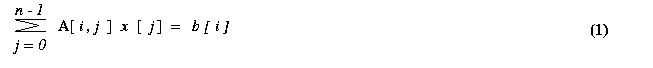
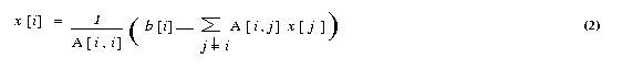
  The Jacobi iterative method is one of the simplest iterative techniques to solve system of linear equations. The i^th equation of a system of linear equations [A]{x}={b} is

  

  If all the diagonal elements of A are nonzero (or are made nonzero by permuting the rows and columns of A), we can rewrite equation (1)

  
  
  

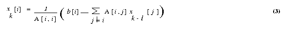
  The Jacobi method starts with an initial guess x₀ for the solution vector x. This initial vector x₀ is used in the right-hand side of equation (2) to arrive at the next approximation x₁ to the solution vector. The vector x₁ is then used in the right hand side of equation (2), and the process continues until a close enough approximation to the actual solution is found. A typical iteration step in the Jacobi method is

  
  

  

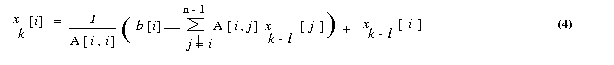
  We now express the iteration step of equation 3 in terms of residual r_k. Equation (3) can be rewritten as

  

  Each process computes n/p values of the vector x in each iteration. These values are gathered by all the processes and each process tests for convergence. If the values have been computed up-to a certain accuracy the iterations are stopped otherwise the processes use these values in the next iterations to compute a new set of values.

• Input

Input Matrix A and Initial Solution Vector x

• Output

solution of matrix system Ax = b

Write a OpenCL program to perform sparse matrix into vector multiplication
(Assignment - To be discussed in Lab. Session)

• Objective

  To write a OpenCL program on sparse matrix multiplication of size n x n and vector of size n.

• Efficient storage format for sparse matrix

  Dense matrices are stored in the computer memory by using two-dimensional arrays. For example, a matrix with n rows and m columns, is stored using a n x m array of real numbers. However, using the same two-dimensional array to store sparse matrices has two very important drawbacks. First, since most of the entries in the sparse matrix are zero, this storage scheme wastes a lot of memory. Second, computations involving sparse matrices often need to operate only on the non-zero entries of the matrix. Use of dense storage format makes it harder to locate these non-zero entries. For these reasons sparse matrices are stored using different data structures. The Compressed Row Storage format (CRS) is a widely used scheme for storing sparse matrices. In the CRS format, a sparse matrix A with n rows having k non-zero entries is stored using three arrays: two integer arrays rowptr and colind, and one array of real entries values. The array rowptr is of size n+1, and the other two arrays are each of size k. The array colind stores the column indices of the non-zero entries in A, and the array values stores the corresponding non-zero entries. In particular, the array colind stores the column-indices of the first row followed by the column-indices of the second row followed by the column-indices of the third row, and so on. The array rowptr is used to determine where the storage of the different rows starts and ends in the array colind and values. In particular, the column-indices of row i are stored starting at colind [rowptr[i]] and ending at (but not including) colind [rowptr[i+1] ]. Similarly, the values of the non-zero entries of row i are stored at values [rowptr[i] ] and ending at (but not including) values [rowptr[i+1] ]. Also note that the number of non-zero entries of row i is simply rowptr[i+1]-rowptr[i].

• Serial sparse matrix vector multiplication

  The following function performs a sparse matrix-vector multiplication [y]={A} {b} where the sparse matrix A is of size n x m, the vector b is of size m and the vector y is of size n. Note that the number of columns of A (i.e., m ) is not explicitly specified as part of the input unless it is required.

  void SerialSparseMatVec(int n, int *rowptr, int *colind, double *values
  double *b, double  *y)   
  { 
        int i, j, count ;  
        count = 0;
        for(i=0; i<n; i++)
        {
          y[i] = 0.0;
          for (j=rowptr[i]; j<rowptr[i+1];   j++)
            y[i] += value [count] * b [colind[j]];
          count ++;
        }
  }
  
  

• Description of parallel algorithm

  In the parallel implementation, each thread picks a row from the matrix and multiplies it with the vector. Thus computation of all threads is carried out in parallel.

• Implementation

  There are two implementations, one using OpenCL kernels and the other using BLAS library.
  
  OpenCL implementation
  
  Step 1: The matrix size(no. of rows) and sparsity(percentage of non-zero) are provided by the user in the cmd line.
  
  Step 2: A sparse matrix and a vector of the given size are allocated and initialized. Also the row_ptr and col_idx vectors are created and assigned their appropriate based on the sparse matrix
  
  Step 3: The above vectors are also created and initialized on the device (Coprocessor).
  
  Step 4: The sparse_matrix and vector are multiplied in the Device (Coprocessor) to obtain the result.
  

• Performance:

  The gettimeofday() function which is part of sys/time.h is used to measure the time taken for computation.

• Input

The input to the problem is given as arguments in the command line. It should be given in the following format ; Suppose that the number of rows of the sparse matrix is n (only square matrices are considered) and the sparsity i.e. the percentage of number of zero's (given in the range 0 to 1) is m, then the program must be run as,

./program_name n m

CPU generates the sparse matrix, the vector to be multiplied using random values and the row_ptr and col_idx vectors based on the sparse matrix.

• Output

The CPU prints the time taken for the computation.

• Objective

  Write OpenCL program to compute addition of two vectors
  

• Description

  We create a one-dimensional globalWorkSize array that is overlaid on vector. The input vectors using Single Precision/Double Precision input data are generated on Host and transfer the vectors to device for vector addition. Each device (Coprocessor) computes addition of its own elements of two vectors and accumalates partial sum. In global memory,a simple kernel based on the one- dimension indexspace of work groups is generated in which work item is given a unique ID within its work group. Each work item performs addition of two vectors using work item ID and the final resultant vector is generated on device and transferred to Host.
  
  Refer Table 1.1 for OpenCL Important implementation Steps

Each work-item using its work item ID performs addition using one element from each vector.

The choice of work-items in the code are given as
size_t globalWorkSize[3] = [128, 1,1];
& for generalisation, refer table 1.2 The number of work-items of workgroup on each Device (Coprocessor) are specified.


• Input

Two vectors of same size

• Output

Execution time in seconds, Gflops achieved